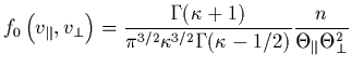
When dealing with non-thermal velocity distributions for the ion species, we must consider the issue of their thermal anisotropy, i.e. the difference in temperature parallel and perpendicular to the magnetic field and the concomitant magnetic mirror force. Unfortunately, the Voyager PLS instrument was only able to measure the perpendicular temperature of the ions. The results reported by Bagenal [1994] were consistent with a perpendicular velocity distribution of the ions having a thermal core with a non-thermal ``tail'' or ``halo''. The Galileo plasma instrument has a full angular response and indicated that the thermal core of the ion distribution is isotropic [ Crary et al., 1998]. In contrast, there is good reason to believe that the halo component of the ion distribution should be highly anisotropic. When neutral atoms (escaped from Io's atmosphere) are first ionized they experience Jupiter's strong magnetic field and ``pick-up'' a gyro-motion perpendicular to the magnetic field equal to the bulk (corotation) speed of the plasma. The initial parallel motion of the pick-up ions is small. Hence, we might expect that a population of freshly-ionized particles would have a highly anisotropic distribution. Eventually, one expects these pick-up ions to be partially thermalized by plasma waves and, on longer time scales, by collisions. While the time scales for partial thermalization of such a ``ring'' distribution are not well known, it is clear that we should expect a substantial anisotropic supra-thermal component for the ion velocity distribution.
For the purposes of modeling an anisotropic distribution having
a suprathermal tail, we adapt an anisotropic kappa distribution from
[ Summers and Thorne, 1992], which we call bi-kappa (by analogy to bi-Maxwellians)
and is of the form:
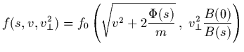
Applying Liouville's theorem with the conservation of energy and
magnetic moment (
![]() ), as in the isotropic
case, one derives the density distribution for each particle species.
Recall that Liouville's theorem allows one to express the
distribution as a function of the curvilinear co-ordinate
), as in the isotropic
case, one derives the density distribution for each particle species.
Recall that Liouville's theorem allows one to express the
distribution as a function of the curvilinear co-ordinate ![]() along
the magnetic field, in the presence of a monotonic attractive
potential
along
the magnetic field, in the presence of a monotonic attractive
potential ![]() , as
, as
By expressing the thermal anisotropy at the equator as
![]() we can use (9) to calculate the moments of the
distributions to derive the latitudinal profiles of density and
temperature as follows:
we can use (9) to calculate the moments of the
distributions to derive the latitudinal profiles of density and
temperature as follows:
When
![]() , one retrieves the results obtained with a
bi-Maxwellian distribution of Huang and Birmingham [1992].
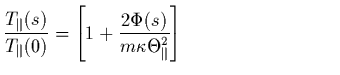
In this case, we get, from equation
12 with
, one retrieves the results obtained with a
bi-Maxwellian distribution of Huang and Birmingham [1992].
In this case, we get, from equation
12 with ![]() (as expected in the torus -see
the above discussion), a perpendicular temperature which decreases
with latitude and, from (11), a constant parallel temperature.
When
(as expected in the torus -see
the above discussion), a perpendicular temperature which decreases
with latitude and, from (11), a constant parallel temperature.
When ![]() (isotropy), one retrieves
the density profile (4) found by
Meyer-Vernet, Moncuquet and Hoang [1995].
(isotropy), one retrieves
the density profile (4) found by
Meyer-Vernet, Moncuquet and Hoang [1995].
Note that with these bi-kappa distributions neither the parallel nor the
perpendicular temperature strictly follow a polytropic law.
The parallel temperature increases with latitude independently of ![]() while
the perpendicular one has an additional variation along the magnetic field
due to the change in
field strength. This means that the anisotropy is not constant along
magnetic field lines, but decreases if
while
the perpendicular one has an additional variation along the magnetic field
due to the change in
field strength. This means that the anisotropy is not constant along
magnetic field lines, but decreases if ![]() . Since the change in
magnetic field strength is small (
. Since the change in
magnetic field strength is small (![]() 20% over the latitudinal range of
Ulysses) this is a minor effect, unless the anisotropy at the
equator is particularly strong.
20% over the latitudinal range of
Ulysses) this is a minor effect, unless the anisotropy at the
equator is particularly strong.
To illustrate the relative effects of the anisotropy and of the suprathermal
tail, we show in Figure 3 several
latitudinal density profiles calculated with different values of the
parameters ![]() and
and ![]() .
.
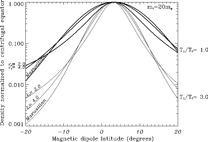 |
The profiles in Figure 3 were obtained by solving
equation (10) for both the electrons and a single ion species with the
equation of charge neutrality
![]() which permits
the elimination of the electric potential
which permits
the elimination of the electric potential ![]() . One can see that
the kappa distributions have the tendency to tightly confine the
particles to the equator while allowing a substantial population at
high latitudes. The effect of increasing the thermal anisotropy
(
. One can see that
the kappa distributions have the tendency to tightly confine the
particles to the equator while allowing a substantial population at
high latitudes. The effect of increasing the thermal anisotropy
(![]() to 3), for either the Maxwellian or kappa cases, is to
further confine the plasma to the equator.
to 3), for either the Maxwellian or kappa cases, is to
further confine the plasma to the equator.
With these tools in hand, including the flexibility of varying the
unknown parameters ![]() and
and ![]() , we are now able to model the
density distributions observed by different spacecraft as they
traversed the torus.
, we are now able to model the
density distributions observed by different spacecraft as they
traversed the torus.
![$\displaystyle \times
\left[ 1+ \frac{v_{\parallel}^{2}}{\kappa \Theta_{\parallel}^{2}}
+ \frac{v_{\perp}^{2}}{\kappa \Theta_{\perp}^{2}}
\right]^{-\kappa -1}$](img105.gif)
![$\displaystyle \frac{n(s)}{n(0)} = {\left[ 1+\frac{2\Phi(s)}{m \kappa
\Theta_{\p...
...right]}
^{\frac{1}{2} - \kappa}
\frac{1}{A_0+(1-A_0)\frac{B(0)}{B(s)}} \protect$](img109.gif)
![$\displaystyle \frac{T_{\perp}(s)}{T_{\perp}(0)} =
{\left[ 1+\frac{2\Phi(s)}{m \...
... \Theta_{\parallel}^2} \right]}
\frac{1}{A_0+(1-A_0)\frac{B(0)}{B(s)}} \protect$](img111.gif)